Sparse Bayesian priors for training variational autoencoders
VAE Overview
Before diving into it, I thought I’d mention that I’ve included a quick refresher on the math behind variational autoencoders (VAE’s) at the end of this article if you’re feeling rusty ;)
Standard VAE’s use normal distributions everywhere, mainly since the math works out nicely when calculating posteriors. I was curious to see how this architecture would behave if instead I changed some underlying assumptions, and modeled the latent space using a spike-and-slab prior.
Under this formulation we assume each latent, $z_{i}$, of the encoded sample, $x$, has some probability, $p$, of being turned “on” or “off”. For $c\in \mathbb{R}$, $|c|<1$ we have for each dimension:
Our goal is to make the VAE learn how to encode and decode samples in a sparse fashion, i.e. where lots of info is “zeroed out”. Sparsity is nice mathematically and in a sec we’ll see what that looks like with a real demo on the MNIST dataset.
It’s important to observe that we can throttle the sparsity through our choice of $p$; $p=1$ means most of the embedding dimensions are uninformative, and $p=0$ recovers the original VAE. The edge cases aren’t that interesting so we’ll take a value in between, $0<p<1$.
We’ll also assume :
- $z_{i}|x \sim \mathcal{N}(\mu_{\phi}(x),\sigma^{2}_{\phi}(x))$
- and $x_{i}|z \sim Be(\theta(z))$.
That last choice is mainly since I’m going to show some examples using grayscale images and we want our generated outputs being a value truncated between 0 and 1.
Okay so here’s the bad news: unfortunately no closed form for the KL-divergence between our mixture model prior and the posterior exists. The good news: we can just estimate the KL loss through Monte Carlo pretty easily:
One last thing, since we’re considering a Bernoulli framework for our probibalistic decoder, the first term in the ELBO breaks down to binary cross entropy (BCE) loss if we assume conditional independence. Indeed,
So we’re looking to minimize the binary cross entropy pixel-wise across the image! We can just use a classic torch.nn.functional.binary_cross_entropy in the code for our reconstruction loss.
Basic PyTorch implementation
Using PyTorch and torch.distributions we can easily implement everything we were just talking about.
First let’s handle the distributional aspects:
assert
=
=
=
=
=
return
# logsumexp :)
= +
= +
return
# k sample monte carlo estimate for kl-divergence
=
return
Now for the loss terms:
, =
= + *
=
#reconstruction loss
=
#kl divergence
=
= 0.8
=
=
=
=
#total loss
= +
I’ve left out the architectures for the encoder and decoder but since the MNIST dataset is fairly simple most choices will do. Notice also that we made use of the LogSumExp trick to handle computing the log probabilities under the spike and slab prior.
With everything in place we can train the model quickly and visualize the resulting embedding space. I’ve left out the training details since this is more a post on the statistics side, but its in line with most tutorials out there.
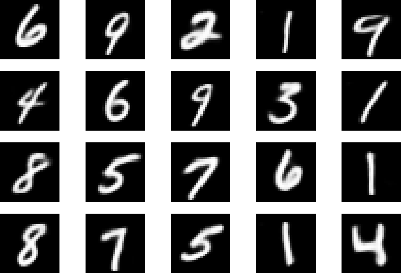
When you train the model you still get a VAE which can produce realistic generations like the ones below, even if we’re using a lossy encoder.
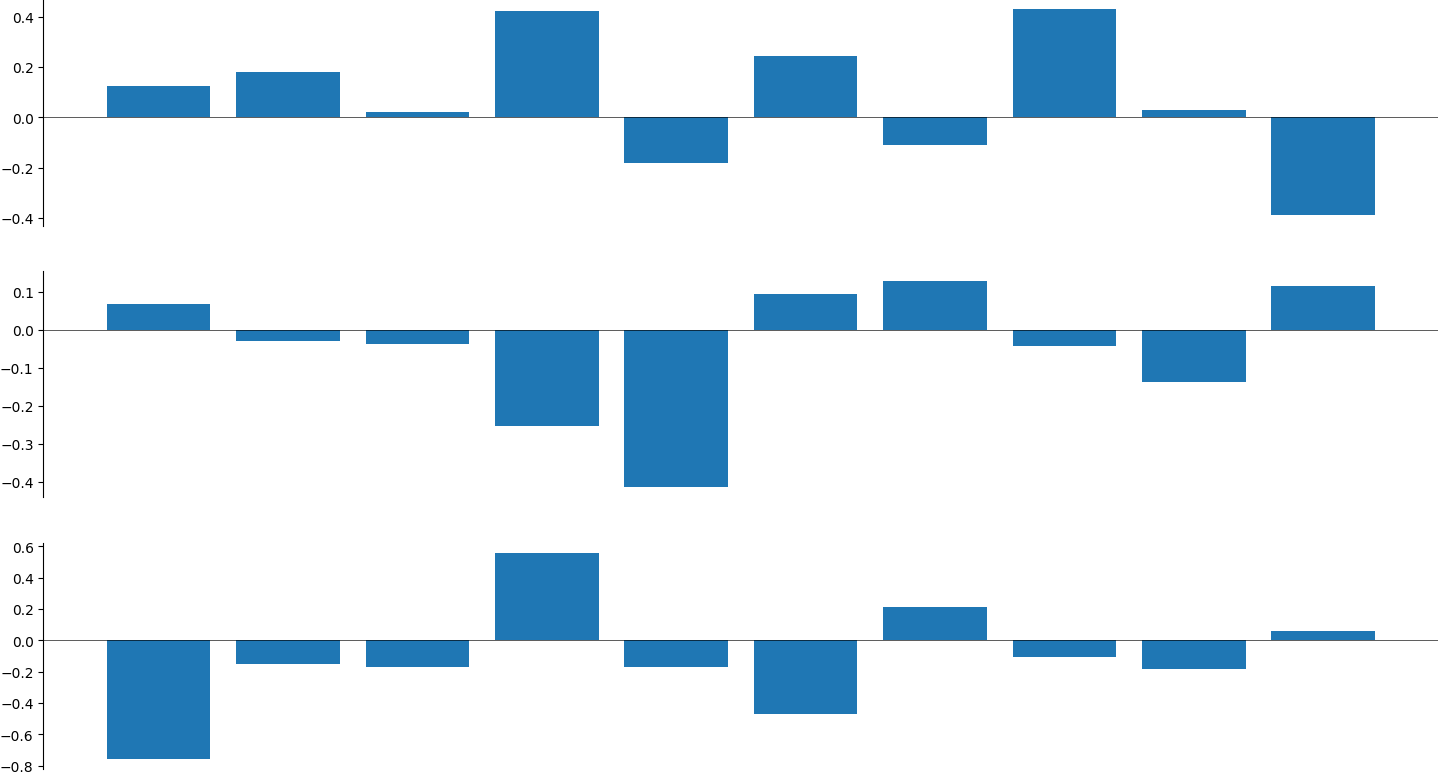
What’s different about this model and the normal VAE is that when we encode images we only have a few non-zero components in the embedding representation. If the embedding space is $d$-dimensional we expect the model to activate only $p*d$ dimensions after training, which we can see by looking at the image below:
There you go! A sparse variational autoencoder which was obtained just from making a few different choices in the statistical scaffolding of the model. I should also note that spike and slab and normal of course aren’t the only choices when designing your VAEs (personal fave of mine is Gumbel Softmax).
Bonus: An in-depth refresher on VAE’s
In terms of the original VAE proposed (rather offhandedly) by Kingma and Welling in 2014, the story goes something like this: suppose we want to learn the underlying distribution for some data (e.g. images) namely for the purpose of generating samples artificially. Just like in GANs we’d like to be able to convert some samples drawn from a parametric distribution into ones which might have come from our real data generator. This is where the probibalistic decoder, $\theta$, comes into play.
The goal of $\theta$ is to map low-dimensional noise into hyperparameters of a parametric distribution which generates realistic high-dimensional samples. Think $x|z \sim f(\theta(z))$
One way to quantify how “good” your decoder is performing is to compute the log probability of a real sample under the decoder framework as
$$ \log p_{\theta}(x) = \log \int_{\mathcal{Z}}p_{\theta}(x,z)dz $$
If your decoder is doing its job, then the probability above should be high under your model.
Since this isn’t a really computationally tractable way to go about things however, another way to express the marginal is through importance sampling w.r.t. the posterior distribution over the latents $z$ given a sample $x$ like
where we’ve assumed that initially $ z\sim p(z) $ (this is the part I’m interested in changing!)
Now this is where the authors got a little sneaky, instead of using the true posterior $p_{\theta}(z|x)$ we can instead come up with a proxy for it through the use of an probibalistic encoder, $\phi$, which turns an input sample into hyperparameters used to model a parametric distribution over the latent space. Think $z|x \sim g(\phi(x))$. With this we write the above as
Now by Jensen’s inequality (just geometry!) you arrive at a lower bound on the likelihood of a sample under our variational autoencoder given by the evidence lower bound.
Therefore maximimzing $\log p_{\theta}(x)$ becomes equivalent to maximizing the ELBO!
Fortunately enough there exists a much nicer representation for the ELBO which is a lot more approachable for us in terms of a numerical optimization perspective; starting (magically) from the KL-divergence between the latent posterior provided by the encoder and the associated prior we get
so that
Hmmm I guess this still looks a bit confusing. To make the case for this model a little bit let's see what happens if we choose to model our probibalistic decoder such that $x|z \sim \mathcal{N}_{n}(\mu_{\theta}(z),1)$.
In this case the first term on the right is proportional toSo that maximizing this term is equivalent to minimizing the reconstruction loss.
By mixing and matching which probibalisitc frameworks you’re operating with for the encoder prior and posterior, and decoder posterior, the form of the ELBO changes accordingly.
References
- Auto-Encoding Variational Bayes by Kingma et al. (2013)
- beta-VAE: Learning Basic Visual Concepts with a Constrained Variational Framework by Higgins et al. (2022)