tl;dr: I trained LLaVA v1.5 7b on a dataset of OCR-aware image captions produced by GPT-4 to improve the base model’s OCR capabilities. With quantization we reduce the model size from 14GB to 4.5GB and accelerate inference by 4x without losing performance.
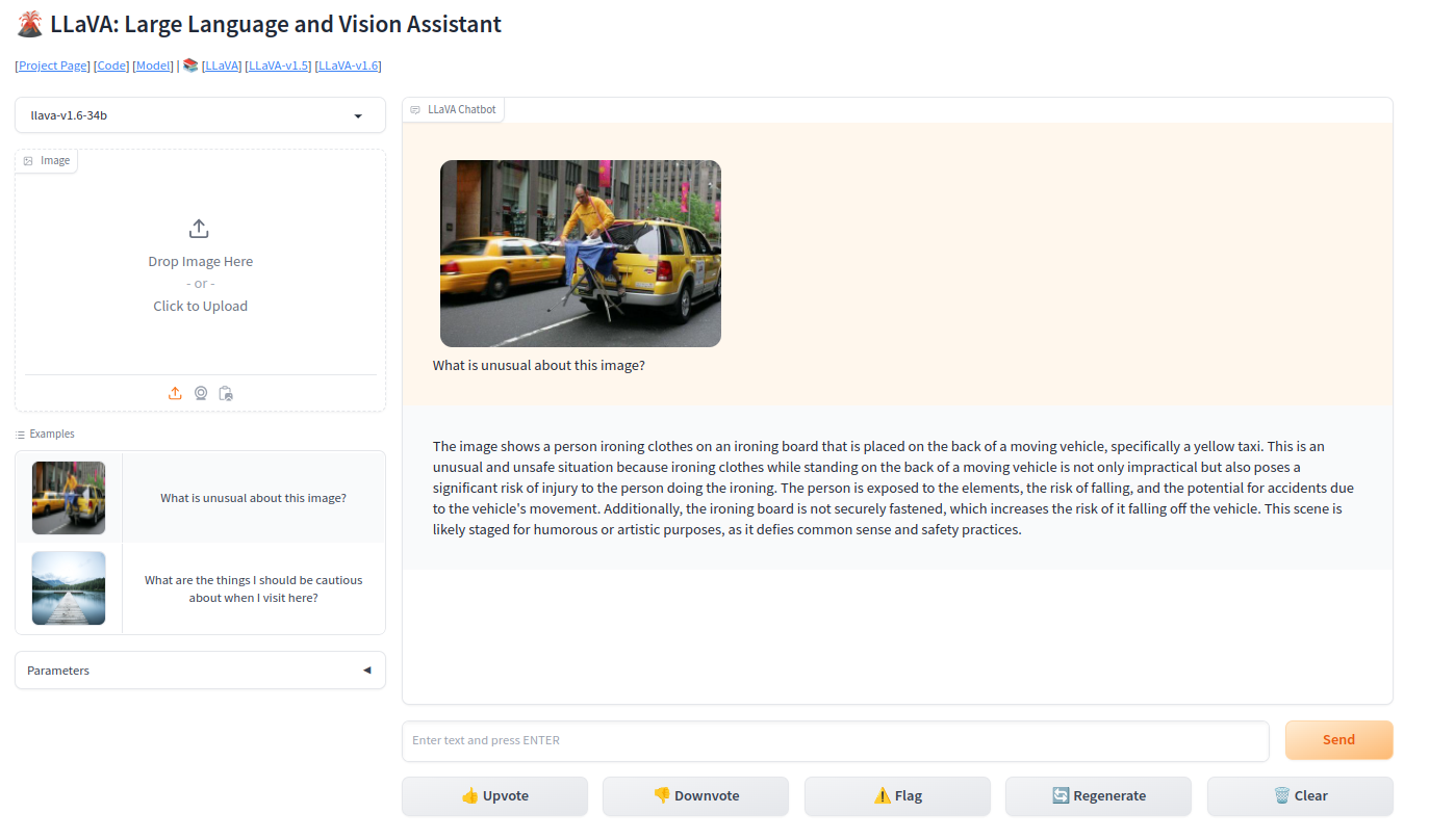
LLaVa is a multimodal model for vision and language that works by combining pretrained vision encoders and LLMs. Since its release in October 2023 its gained a lot of traction in the community as a solid open-source alternative to GPT-4, with many projects quickly providing support for model inference in their platforms and allowing users to deploy LLaVA locally.
In this article, we will run through the pipeline of training and quantizing a 7b-variant of LLaVA on a custom dataset. The goal is to end up with a smaller version of the base model with improved performance on OCR-related tasks.
🌋 Introduction to LLaVA
The model works by training small projection layer between CLIP and the LLM so that vision tokens prefix the inputs to the language model. Its a lot simpler than other approaches in the past like BLIP/InstructBLIP or Flamingo and in practice works a lot better too!
The key contributions of the authors in the original paper was that LLMs like GPT3.5/4 can be prompted to create high quality visual instruction tuning datasets which allow smaller models to mimic GPT-like performance.

During training both the vision encoder and LLM are kept frozen while the projection layer learns to align the visual concepts with the LLM’s embedding space. In the original model we used only LLMs with a llama backbone (e.g. llama2 chat or vicuna) in the 7b and 13b variants, but in the latest release support has been provided for newer architectures like Mistral.
I’ll be training the 7b version with vicuna as the llm backbone.
🏋️ Resource-efficient training
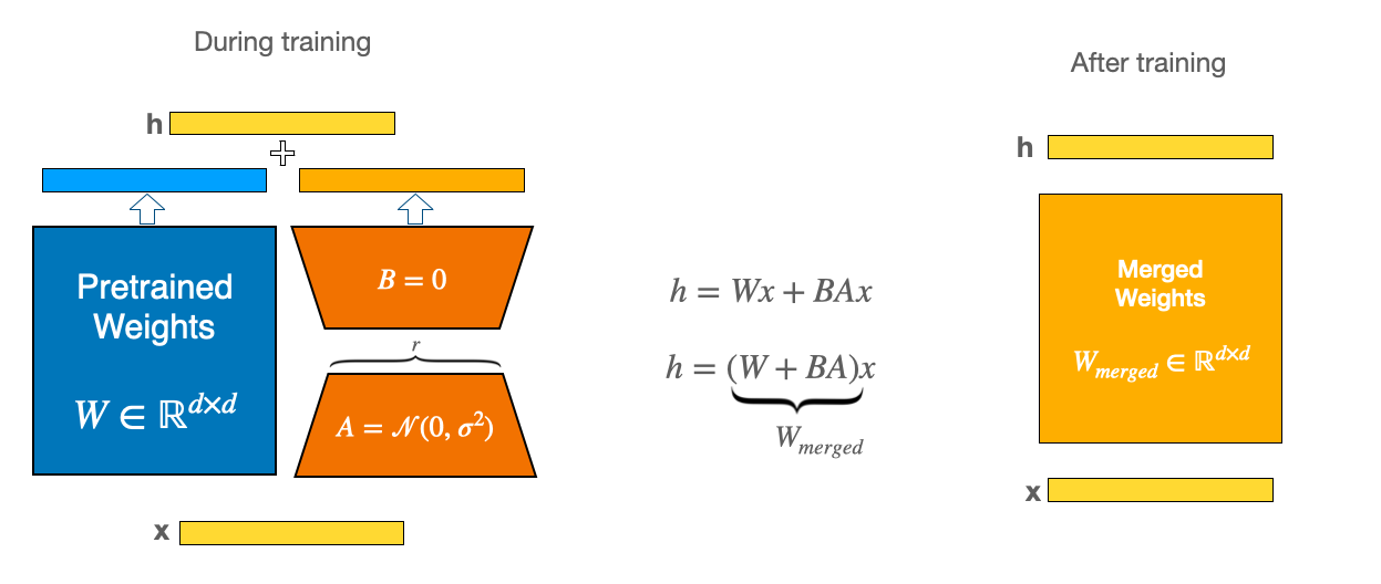
When we finetune LLaVA, we’ll be making use of LoRA/QLoRA to inject a few low-rank trainable matrices at key layers in the LLM so that only a small fraction of the weights are unfrozen (generally less than 1%). This way we’ll be able to fit the model on consumer-grade GPUs without running into a CUDA oom. In my case I have access to a 4xL4 node which gives me around 96GB of VRAM to work with so I’ll be using normal LoRA. If in your case you’re more limited on GPU memory QLoRA is your best bet.
To showcase why we need training tricks like LoRA, let’s quickly estimate the memory requirements of a full fine-tuning for the model we’ll be considering, llava-v1.5-7b. First we can count the number of parameters in the model using the code below (make sure transformers>=4.36 is installed):
import torch
from transformers import LlavaForConditionalGeneration

model_id = "llava-hf/llava-1.5-7b-hf"
model = LlavaForConditionalGeneration.from_pretrained(model_id, torch_dtype=torch.float16)
n = sum(p.numel() for p in model.parameters()) # 7063427072
In addition to the parameters themselves, we also need to store activations and optimizer states. If we’re using standard AdamW the cost is 8 bytes per parameter, while for the parameters and activations we’re looking at another 4 bytes per param in full precision training. With this the calculation looks like GB = 105.25 GB. Even in half precision this is still 52.625 GB which is over 3x the memory you can get in a free Google Colab session.
As a sanity check we can also use the accelerate cli tool for estimating memory usage for the base llm, which for us will be vicuna-7b-v1.5 as follows:
$ pip install accelerate
$ accelerate estimate-memory lmsys/vicuna-7b-v1.5 --library_name transformers

>Loading pretrained config for `lmsys/vicuna-7b-v1.5` from `transformers`...
┌────────────────────────────────────────────────────┐
│  Memory Usage for loading `lmsys/vicuna-7b-v1.5`   │
├───────┬─────────────┬──────────┬───────────────────┤
│ dtype │Largest Layer│Total Size│Training using Adam│
├───────┼─────────────┼──────────┼───────────────────┤
│float32│  776.03 MB  │ 24.74 GB │      98.96 GB     │
│float16│  388.02 MB  │ 12.37 GB │      49.48 GB     │
│  int8 │  194.01 MB  │ 6.18 GB  │        N/A        │
│  int4 │   97.0 MB   │ 3.09 GB  │        N/A        │
└───────┴─────────────┴──────────┴───────────────────┘
Since we’re training a vision encoder + a projection layer on top of vicuna we expect the requirements to be higher than the base LLM which is what we can see from the above. Using LoRA though with some default settings we can see how small the requirements become:
# make sure peft installed

# --- snip  ---
from peft import PeftModel, LoraConfig

lora_config = LoraConfig(
    r = 8,
    lora_alpha = 256,
    target_modules = ['q_proj','k_proj','v_proj','o_proj','up_proj','down_proj'],
)

peft_model = PeftModel(model, lora_config)
peft_model.print_trainable_parameters()
> trainable params: 17,301,504 || all params: 7,080,728,576 || trainable%: 0.2443463806626218With this new configuration we’re only training 0.244% of the original parameters!
If you’re inclined to tweak the source code a bit to add more memory-efficient techniques like GaLore, or low-bit optimizers you can probable eke out a bit more performance from your GPU. For this article though I won’t be touching the internals of the training repo.
👾 GPT-4 OCR annotations
One limitation of LLaVA is its performance on OCR-related tasks. This is due mainly to the fact that the input image resolution is 336x336 and also since the majority of the training data is more geared towards caption generation and VQA. I want to see if we can improve upon the baseline using a dataset of OCR-aware captions generated by GPT-4 that the model did not see during training.
To get a baseline feel for kind of outputs our model generates before finetuning, lets run an example inference real quick:
# --- snip ---
import requests
from PIL import Image
from transformers import AutoProcessor
from dataclasses import dataclass

processor = AutoProcessor.from_pretrained(model_id)

url = "https://www.nartakmediagroup.com/wp-content/uploads/2023/12/Screen-Shot-2023-12-20-at-5.05.06-PM.webp"
image = Image.open(requests.get(image_file, stream=True).raw).convert("RGB")
prompt = "USER:<image>\ndescribe this image.\nASSISTANT: "

inputs = processor(prompt, image, return_tensors = 'pt').to(0, torch.float16)

@dataclass
class GenerationArguments:
    min_new_tokens: int = 1
    max_new_tokens: int = 256
    temperature: float = 0.8
    do_sample: bool = True
    num_beams: int = 1
    num_return_sequences: int = 1

model.generate(
            **inputs,
            **asdict(generation_config),
        )

print(processor.tokenizer.batch_decode(out[:,len(processor.tokenizer.encode(args.prompt)):], skip_special_tokens = True)[0])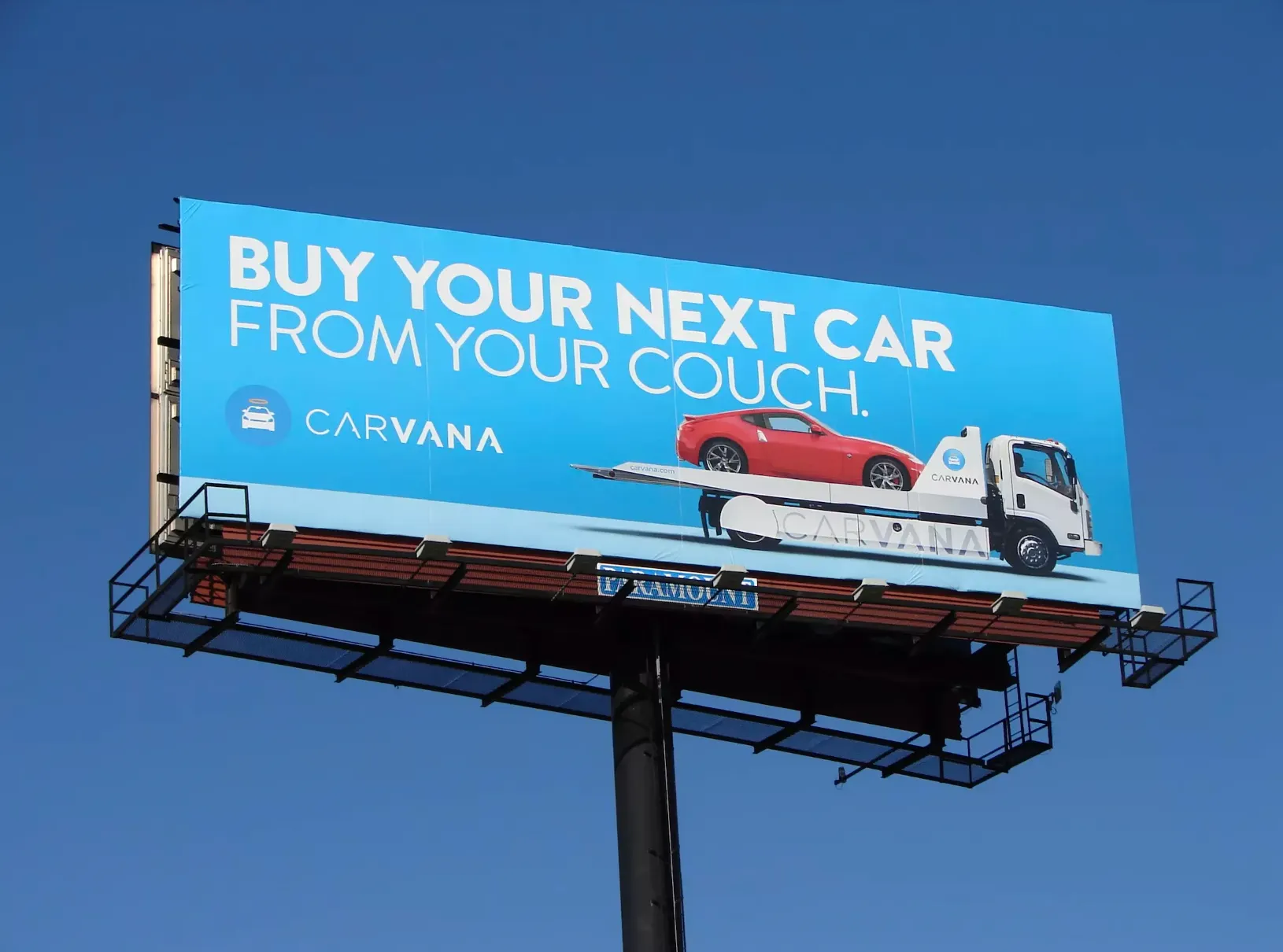
A large billboard advertises a red sports car being transported by a tow truck.
The model didn’t make any comments on the big text in the centre of the image and overall isn’t very descriptive. Let’s see if we can improve on that!
⚙️ Fine-tuning on custom data
The entire training pipeline for LLaVA works out-of-the-box using the official repo with parameters for memory efficient training like micro-batching, activation checkpointing, FSDP, and LoRA being configured directly from the launch script.
We first start by cloning the repo and making the virtual environment:
$ git clone git@github.com:haotian-liu/LLaVA.git
$ cd LLaVA
$ conda create -n llava python=3.10 -y
$ conda activate llava
$ pip install --upgrade pip && pip install -e ".[train]"
To get our data in the expected training format we first need to download the images from Meta. Once those are downloaded we can resolve the names with those in the hugging face one.
# make sure `datasets` installed
from datasets import load_dataset
from uuid import uuid4
import json

dataset = load_dataset("jimmycarter/textocr-gpt4v", split='train')

def preprocess(examples):
    text = examples['caption_condensed']
    filenames = examples['filename']
    llava = [{
        'id': str(uuid4()),
        'image':f,
        'conversations':[
            {
                'from':'human',
                'value':'<image>\nDescribe this image in detail.'
            },
            {
                'from': 'gpt',
                'value': t
            }
        ]} for f,t in zip(filenames, text)]

    examples['llava'] = llava
    return examples

dataset = dataset.map(preprocess, batched=True, remove_columns=dataset.columns)

path = #your/path/to/dataset.json
with open(path, 'w') as f:
    f.write(json.dumps(dataset['llava']))
Now the only thing left to do is configure the training script and we’re good to go! An example script can be found in LLaVA/scripts/v1_5/finetune_task.sh. Notice how some options can be explicitly configured to improve memory efficiency:
--lora_enable True --lora_r 48 --lora_alpha 256 --mm_projector_lr 2e-5 \
--deepspeed ./scripts/zero3.json \
--bf16 True \
--gradient_checkpointing True \
--per_device_train_batch_size 1 \
If you don’t have the model checkpoints cached already the code will handle downloading the llm and vision encoder weights for you when you train. The full training script I’ll be using is included below.
#!/bin/bash

deepspeed llava/train/train_mem.py \
    --lora_enable True --lora_r 48 --lora_alpha 256 --mm_projector_lr 2e-5 \
    --deepspeed ./scripts/zero3.json \
    --model_name_or_path lmsys/vicuna-7b-v1.5 \
    --version v1 \
    --data_path ./dataset.json \
    --image_folder ./images \
    --vision_tower openai/clip-vit-large-patch14-336 \
    --mm_projector_type mlp2x_gelu \
    --mm_vision_select_layer -2 \
    --mm_use_im_start_end False \
    --mm_use_im_patch_token False \
    --image_aspect_ratio pad \
    --group_by_modality_length True \
    --bf16 False \
    --fp16 True \
    --output_dir ./checkpoints/llava-v1.5-7b-lora-gpt4OCR \
    --num_train_epochs 1 \
    --per_device_train_batch_size 1 \
    --per_device_eval_batch_size 4 \
    --gradient_accumulation_steps 4 \
    --evaluation_strategy "no" \
    --save_strategy "epoch" \
    --save_total_limit 1 \
    --learning_rate 2e-4 \
    --weight_decay 0. \
    --warmup_ratio 0.03 \
    --lr_scheduler_type "cosine" \
    --logging_steps 1 \
    --model_max_length 2048 \
    --gradient_checkpointing True \
    --dataloader_num_workers 4 \
    --lazy_preprocess True \
    --report_to wandb
We launch the script from inside the repo with:
$ source ./scripts/v1_5/finetune_task.sh🚀 Results
After training the model with LoRA and the above settings for one epoch we can already see a huge qualitative difference in the type of outputs our model yields. Asking the same question to the model as before for the image of the billboard, our newly-generated response is much more OCR-aware and descriptive:
The billboard advertisement showcases a red sports car being towed by a Carvana truck, with the slogan “Buy your next car from your next couch.” The Carvana logo is prominently displayed in the top right corner, and the Carvana website is noted in the bottom right corner of the billboard.
Nice! Now we can focus on making the finetuned model with the new weights available in different quantized formats.
🤏🏼 Quantization
 Example inference for our fine-tuned llava quantized with autoawq
By changing the precision in which we store the model weights we can dramatically cut down on the model’s memory footprint and also actually gain in terms of inference speed.
I’ve included a summary of the main quantization techniques we’ll consider below. For each of the methods listed I strongly encourage you to check out the source projects and understand how they work under the hood, some of them can get a bit confusing but generally speaking the strategy is usually intuitive.
| Method | Comments | GPU | CPU |
|---|---|---|---|
| GGUF |
| ✅ | ✅ |
| AWQ |
| ✅ | ✅ |
| BnB |
| ✅ | ❌ |
| HQQ |
| ✅ | ✅ |
I won’t run through a step-by-step of how to use each method since it’s quite repetitive but I’ll point you in the direction of the main resources I used along the way:
- GGUF
- AWQ
- BnB
- HQQ
NOTE: In order to quantize using AWQ or HQQ the model needs to be converted into the huggingface format using llava/quantize/convert_llava_weights_to_hf.py script from the transformers repo.
To show the effect of each different technique I prompted each quantized model to answer the same question we were considering before and benchmarked decoding speed along with model size.
| method | size (GB)↓ | speed (tokens/sec)↑ |
|---|---|---|
| q2_k (gguf) | 2.53🥇 | 3.85 |
| hqq (2bit, group size 64) | 3.73 | 8.4 |
| q4_k_m (gguf) | 4.08 | 4.43 |
| hqq (4bit, group size 64) | 4.11 | 7.3 |
| awq | 4.54 | 22.7🥇 |
| nf4 (bnb) | 5.0 | 15.8 |
My personal favourite is the quant generated by AWQ due to its speedy inference and medium size of 4.5GB. It also goes without saying that there’s generally a tradeoff between model size and llm coherence, with smaller quants like q2_k yielding strangely phrased and incoherent outputs. That being said, the algorithm HQQ employs for quantization seems to result in much more stable models with their 2bit quant being as accurate as models twice its size.
Just for fun I figured I’d include the different outputs each quantized model generated down below:
| method | generation |
|---|---|
| q2_k (gguf) | The image features an advertisement billboard with a vibrant red car being transported by trucks, set against a clear sky backdrop. Emblazoned across the top is the phrase “Buy your next CAR from your COUCH.” Below, the text reads “CARVANA” on the left and “carvana” on the right side, while a smaller “Bluegrass Outdoor” logo is noted at the bottom center. |
| hqq (2bit, group size 64) | The billboard advertisement showcases a red sports car being towed by a Carvana truck, with the slogan “Buy your next car from your next couch.” The Carvana logo is prominently displayed in the top right corner, and the Carvana website is noted in the bottom right corner of the billboard. |
| q4_k_m (gguf) | The image depicts an advertisement billboard against a blue sky backdrop, displaying an orange car being transported on a flatbed truck emblazoned with the word “CARVANA.” Below the central message reading “BUY YOUR NEXT CAR FROM YOUR COUCH. CARVANA,” the text “Carvana” is prominently displayed in both yellow and white fonts, while a small “e” logo is also noticeable at the bottom right corner of the billboard. |
| hqq (4bit, group size 64) | The image features a billboard advertisement for Carvana, showcasing a red sports car being towed on a flatbed truck, with the slogan “BUY YOUR NEXT CAR FROM YOUR COUCH. CARVANA” prominently displayed at the top. The billboard also includes the Carvana logo and the website “CARVANA.COM” at the bottom. |
| awq | The image captures a Carvana billboard under a clear blue sky, showcasing a red sports car being towed by a white Carvana truck. The billboard prominently features the Carvana logo and the slogan “Buy your next car from your couch”. |
| nf4 (bnb) | The image features a billboard advertisement for Carvana, showcasing a red sports car being transported on a flatbed truck, with the slogan “BUY YOUR NEXT CAR FROM YOUR COUCH” prominently displayed at the top. The Carvana logo is prominently featured in the center of the billboard, and the word “Carvana” is repeated at the bottom. The billboard is set against a clear blue sky. |
Conclusion
In this article we showed how to finetune LLaVA on a custom dataset to align model generations with an expected format. Even though there are limitations in terms of the input image resolution, we saw that by using a rich dataset of OCR-aware annotations generated by GPT-4 we can teach LLaVA to produce similar high-quality and descriptive outputs. Finally, by quantizing the model with different techniques we were able to cut down significantly on the memory footprint without compromising on performance.
Thanks for reading the article. I encourage you to train the model on your own custom datasets and explore which quantization format is right for your usecase.
References
- Visual Instruction Tuning by Liu et al. (2023)
- LoRA: Low-Rank Adaptation of Large Language Models by Hu et al. (2023)
- QLoRA: Efficient Finetuning of Quantized LLMs by Dettmers et al. (2023)
- AWQ: Activation-aware Weight Quantization for LLM Compression and Acceleration by Lin et al. (2023)